İzmir Reservoir and Water Consumption Forecasting
A four-person team project that assembled ten years of a city's water data into one monthly table, and forecast reservoir occupancy from it.
What it is A monthly model of İzmir's reservoir occupancy and water consumption, built from ten years of public municipal and meteorological data.
What I built The data preparation and integration, the feature engineering, the model comparison, and the weather gap-filling that made the table usable.
My role
This was a four-person project and the narrative below says "we" where the work was shared. My own contribution was the data and the modelling: cleaning and preparing the raw series, integrating the separate datasets into one monthly table, the feature engineering, training the models, comparing and evaluating them, and the visualisation. I wrote the Meteostat gap-filling step that replaced the missing weather months with real station observations. I also prepared the final presentation and presented the project.
01
Ten years of a city's water, one row a month
İzmir publishes its water data. It does not publish it in one place, in one shape, or at one interval.
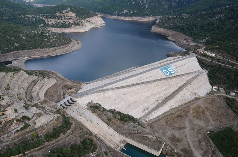
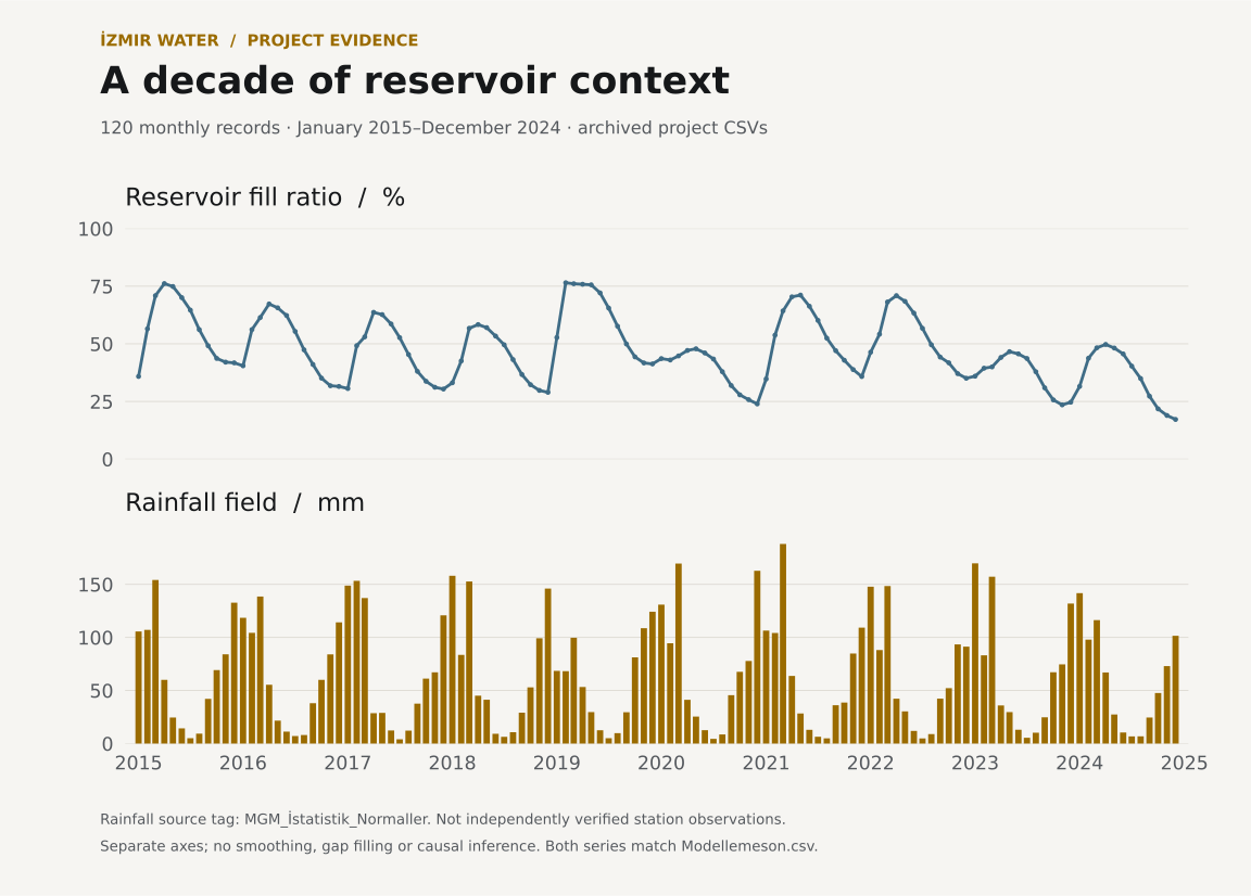
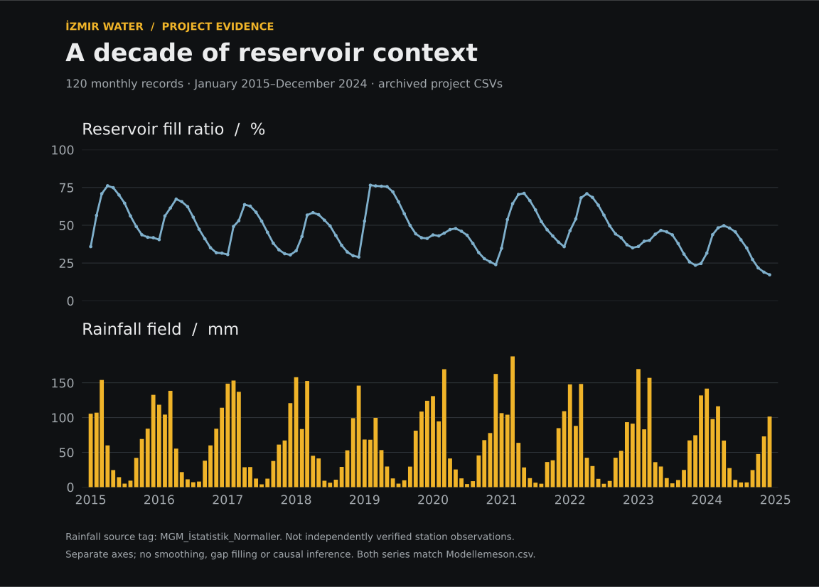
İzmir’s reservoirs, the water the city consumes and the weather that drives both are all a matter of public record. They are published by different bodies, in different formats, at different intervals, and some of it arrives as tables inside annual reports instead of as data.
We set out to put ten years of it into a single monthly table and see how well reservoir occupancy could be forecast from it. That is the kind of indicator a water utility could act on. We wanted an error small enough to be worth quoting and a model simple enough to explain to the person acting on it.
The scope that came out of that is deliberately narrow. One city, one decade, one row per month.
- Period 2015-01 to 2024-12, 120 monthly rows
- Targets Reservoir occupancy (%) and stored volume (m³)
- Inputs Consumption, production, population, temperature, rainfall, humidity, pressure, wind
- Consumption sources İZSU subscription and consumption records, 2014 to 2024
- Weather sources Turkish State Meteorological Service statistics, gap-filled from Meteostat stations
The assembled monthly table is public. It was published to Kaggle by one of the team, and it is the same table the numbers on this page were produced from.

02
Where the numbers came from, and where they did not
Every column in the table can name its source. That was the point of the table.
Merging public series is mostly a bookkeeping problem, and bookkeeping is where this kind of project quietly goes wrong. A value that was estimated, a month that was interpolated and a month that was measured all look identical once they are in the same column. So we carried the provenance in the data instead of in someone’s memory. The consumption rows name the İZSU report they came from, the weather rows name the station, and the gap-filled months name the service and the coverage window they were filled from.
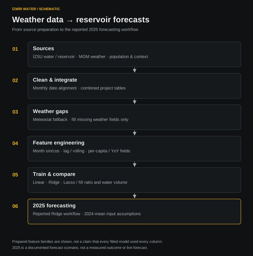
The weather series had holes in it. Interpolating across them would have invented values and hidden the fact, so I pulled the missing months from Meteostat’s station records for İzmir instead. The Çiğli station comes first, with Adnan Menderes as the fallback. Where relative humidity was absent but temperature and dew point were present, it is derived with the Magnus formula instead of being left empty.
Two rules in that step are the ones worth stating. It fills only what is missing, so a real observation is never overwritten by a substitute. And it writes a provenance note into the output, so the next person to open the file learns where those months came from without having to ask anyone.
fill_izmir_real_meteostat.py
for target in [col_prcp, col_nem, col_pres, col_wspd]:
  source = target + '_ms'
    # Fill ONLY the gaps — never overwrite a real observation.
  mask = df[target].isna() & df[source].notna()
  df.loc[mask, target] = df.loc[mask, source]

df['Kaynak_Notu'] = (
  "Real monthly values. Source: Meteostat monthly/hourly dumps. "
  "Station priority: Çiğli (17218) -> Adnan Menderes (17219). "
  "Coverage: 2015-01 .. 2024-12."
)
Only NaNs are touched, and the file records what was done to it.
Not every column earned that confidence. The table carries a split of consumption into domestic, industrial and agricultural use, and a monthly consumption total. Both are derived: the split is one fixed ratio applied to every month, and the monthly total is the daily figure times thirty. They are useful for shaping a model and they are not measurements, so we do not quote them as results anywhere, here or in the presentation.
03
Why the simple model won
120 rows, strong seasonality, and a target that mostly depends on where it was last month.
The features that mattered were the ones that encode time. Month went in as a pair of cyclical terms instead of a plain number, so that December and January sit next to each other instead of eleven apart. The previous month’s value and a three-month rolling mean went in as lag features. Season went in one-hot. Population was added per capita and as a year-on-year change, and we tested a tourist-count feature to see whether summer visitors explained anything the calendar did not.
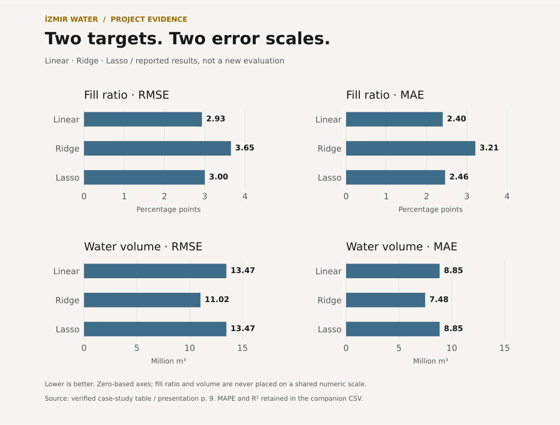
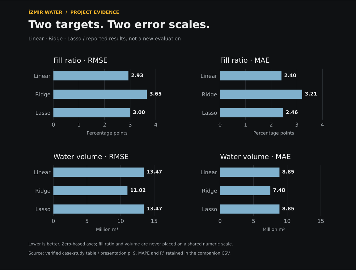
We evaluated linear, ridge and lasso regression against random forest and gradient boosted trees. On this dataset the regularised linear models came out better, and they did so consistently across both targets.
| Model | Target | RMSE | MAE | MAPE | R² |
|---|---|---|---|---|---|
| Linear | Occupancy % | 2.93 | 2.40 | 6.74% | 0.913 |
| Lasso | Occupancy % | 3.00 | 2.46 | 6.87% | 0.909 |
| Ridge | Occupancy % | 3.65 | 3.21 | 9.14% | 0.866 |
| Ridge | Volume m³ | 11.02M | 7.48M | 2.58% | 0.938 |
| Linear | Volume m³ | 13.47M | 8.85M | 3.01% | 0.908 |
| Lasso | Volume m³ | 13.47M | 8.85M | 3.01% | 0.908 |
That is not because trees are worse in general. 120 monthly rows is very little data, and almost all of the structure in this target is seasonality plus where the series was last month. A linear model with cyclical and lag terms represents that directly. An ensemble has to rediscover it from the data, and there is not enough data here for it to do so reliably.
One honest footnote. Our linear and ensemble runs were scored on different train and test splits, so the two sets of error figures are not a controlled comparison. They support the decision we took on this dataset. They do not support a general claim about either family of models.
We also wrote down what would change the answer. Weekly or daily data instead of monthly, an error that starts drifting, a non-linear pattern left in the residuals, or a genuinely new input such as evaporation or inflow would each be a reason to revisit the ensembles.
04
Forecasting the year ahead
A model is only useful if somebody can run it forward.
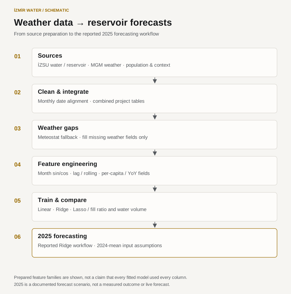
For the 2025 projection we trained ridge regression on the full ten years, then rolled the model forward. The lag and rolling features for each month of 2025 are computed from the tail of 2024. The inputs that cannot be known in advance are temperature, rainfall and population, and those are filled with 2024 averages.
That last choice is a placeholder and not a forecast. It is the right shape for showing how the model behaves over a year, and it means the projection inherits whatever 2024’s weather happened to be. A real operational version would take those inputs from a meteorological forecast. That is where I would take this next, along with an automated pipeline for the reservoir data instead of the manual collection we did here.

What the finished work does
- Merges five public monthly series for İzmir into one table, 2015 to 2024
- Records the source of every column, including which months were gap-filled and from where
- Fills missing weather months from real station observations, never overwriting a measured value
- Builds cyclical month, lag, rolling-mean, per-capita and year-on-year features
- Compares linear, ridge and lasso regression against random forest and gradient boosting on both targets
- Reports MAE, RMSE, MAPE and R² for each model and target
- Projects reservoir occupancy across 2025 from a ridge model trained on the full period
Where the limits are
Two columns in the assembled table are derived, not measured, and nothing on this page treats them as findings. The split between domestic, industrial and agricultural use is a fixed ratio applied to every month, not a measured breakdown; and monthly consumption is the daily figure multiplied by thirty, not an independently metered monthly total. The model comparison has a real caveat too: the linear and the ensemble experiments were scored on different train and test splits, so the gap between them is a reason to prefer the simple model on this dataset, not a controlled measurement of one beating the other. With 120 rows there was no room for a separate validation set, and the 2025 forecast fills its weather and population inputs with 2024 averages. That is a reasonable placeholder and not a weather forecast.
Evidence on this page: Public dataset · Source code · Generated output